Poor Conditioning

Conditioning refers to how rapidly a function changes with respect to small changes in its inputs. Functions that change rapidly when their inputs are perturbed slightly can be problematic for scientific computation because rounding errors in the inputs can result in large changes in the output. Consider the function $$f(x) = A^{-1}x$$. When $$A \in R^{n \times n}$$ has an eigenvalue decomposition, its condition number is

$$ max_{i,j} |\frac {\lambda_i} {\lambda_j}|

$$

This is the ratio of the magnitude of the largest and smallest eigenvalue. When this number is large, matrix inversion is particularly sensitive to error in the input. This sensitivity is an intrinsic property of the matrix itself, not the result of rounding error during matrix inversion. Poorly conditioned matrices amplify pre-existing errors when we multiply by the true matrix inverse. In practice, the error will be compounded further by numerical errors in the inversion process itself.

Gradient-Based Optimization

Most deep learning algorithms involve optimization of some sort. Optimization refers to the task of either minimizing or maximizing some function f (x) by altering x. We usually phrase most optimization problems in terms of minimizing f (x). Maximization may be accomplished via a minimization algorithm by minimizing −f ( x ) . The function we want to minimize or maximize is called the objective function or criterion . When we are minimizing it, we may also call it the cost function, loss function , or error function . We often denote the value that minimizes or maximizes a function with a superscript ∗ . For example, we might say $$x ^∗ = arg min f ( x ) $$

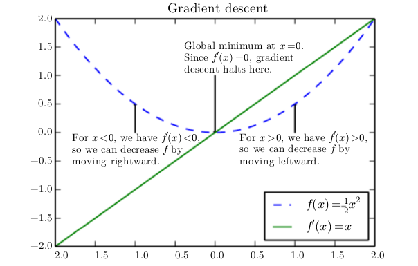
Suppose we have a function y = f (x), where both x and y are real numbers. The derivative of this function is denoted as$$f^{'}(x)$$ or as $$\frac{dy}{dx}$$. The derivative $$f^{'}(x)$$ gives the slope of f (x) at the point x. In other words, it specifies how to scale a small change in the input in order to obtain the corresponding change in the output: $$f(x+\epsilon) \approx f(x) + \epsilon f^{'}(x)$$.

The derivative is therefore useful for minimizing a function because it tells us how to change x in order to make a small improvement in y. For example, we know that $$f(x-\epsilon * sign(f^{'}(x)))$$ is less than f(x) for small enough $$\epsilon$$. We can thus

reduce f (x) by moving x in small steps with opposite sign of the derivative. This technique is called gradient descent (Cauchy , 1847 ).

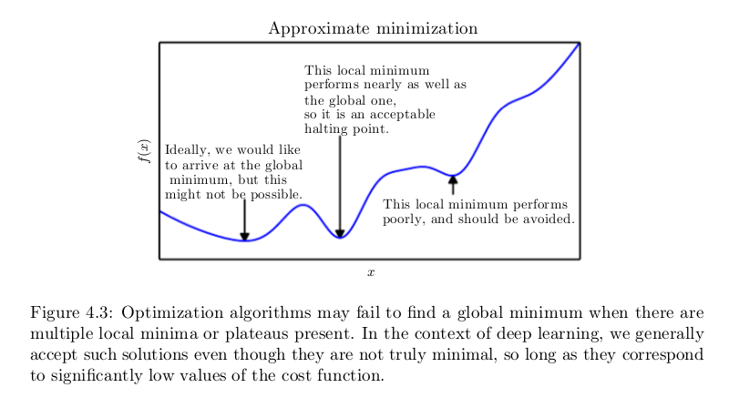
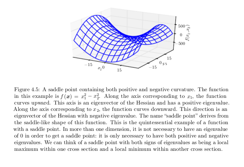
When $$f^{'}(x) = 0$$, the derivative provides no information about which direction to move. Points where $$f^{'}(x) = 0$$ are known as critical points or stationary points . A local minimum is a point where f(x) is lower than at all neighboring points, so it is no longer possible to decrease f (x) by making infinitesimal steps. A local maximum is a point where f(x) is higher than at all neighboring points, so it is not possible to increase f(x) by making infinitesimal steps. Some critical points are neither maxima nor minima. These are known as saddle points.

A point that obtains the absolute lowest value of f (x) is a global minimum. It is possible for there to be only one global minimum or multiple global minima of the function. It is also possible for there to be local minima that are not globally optimal. In the context of deep learning, we optimize functions that may have many local minima that are not optimal, and many saddle points surrounded by very flat regions. All of this makes optimization very difficult, especially when the input to the function is multidimensional. We therefore usually settle for finding a value of f that is very low, but not necessarily minimal in any formal sense.

Multi Dimension

We often minimize functions that have multiple inputs: $$f: R^n \to R$$. For the concept of “minimization” to make sense, there must still be only one (scalar) output.

For functions with multiple inputs, we must make use of the concept of partial derivatives. The partial derivative $$\frac {\partial} {\partial x_i} f(x)$$ measures how f changes as only the variable $$x_i$$ increases at point x. The gradient generalizes the notion of derivative to the case where the derivative is with respect to a vector: the gradient of f is the vector containing all of the partial derivatives, denoted $$\triangledown_x f(x)$$. Element i of the gradient is the partial derivative of f with respect to $$x_i$$ . In multiple dimensions, critical points are points where every element of the gradient is equal to zero.

The directional derivative in direction u (a unit vector) is the slope of the function f in direction u. In other words, the directional derivative is the derivative of the function f (x + αu) with respect to α , evaluated at α = 0. Using the chain rule, we can see that

$$ \frac {\partial} {\partial \alpha} f(x+ \alpha u) = u^T \triangledown_x f(x)

$$

To minimize f , we would like to find the direction in which f decreases the fastest. We can do this using the directional derivative:

$$ min{u, uu^t=1} u^T\triangledown_xf(x) = min{u, uu^T=1} \parallel u \parallel_2 \parallel \triangledown_x f(x) \parallel_2 \cos(\theta)

$$

where θ is the angle between u and the gradient. Substituting in $$\parallel u \parallel_2 = 1$$and ignoring factors that do not depend on u, this simplifies to $$min_u \cos(\theta)$$. This is minimized when u points in the opposite direction as the gradient. In other words, the gradient points directly uphill, and the negative gradient points directly downhill. We can decrease f by moving in the direction of the negative gradient. This is known as the method of steepest descent or gradient descent .

Steepest descent proposes a new point $$x ^ {'} = x - \epsilon \triangledown_x f(x)$$, where $$\epsilon$$ is the learning rate, a positive scalar determining the size of the step. We can choose $$\epsilon$$ in several different ways. A popular approach is to set $$\epsilon$$ to a small constant. Sometimes, we can solve for the step size that makes the directional derivative vanish. Another approach is to evaluate $$f(x-\epsilon \triangledown_x f(x))$$ for several values of $$\epsilon$$ and choose the one that results in the smallest objective function value. This last strategy is called a line search.

Steepest descent converges when every element of the gradient is zero (or, in practice, very close to zero). In some cases, we may be able to avoid running this iterative algorithm, and just jump directly to the critical point by solving the equation ∇ x f ( x ) = 0 for x .

Jacobian Matrices

Sometimes we need to find all of the partial derivatives of a function whose input and output are both vectors. The matrix containing all such partial derivatives is known as a Jacobian matrix. Specifically, if we have a function $$f: R^m \to R^n$$ , then the Jacobian matrix $$J \in R^{n*m}$$of f is defined such that $$J_{i,j} = \frac {\partial} {\partial x_j} f(x)_i$$ .

Second Derivative and Curvature

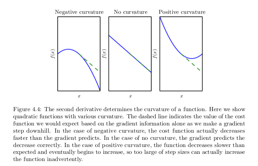
We are also sometimes interested in a derivative of a derivative. This is known as a second derivative. For example, for a function $$f: R^n \to R$$, the derivative with respect to $$x_i$$ of the derivative of f with respect to$$x_j$$ is denoted as $$\frac {\partial^2} {\partial x_i \partial x_j} f$$ . In a single dimension, we can denote $$x = y$$$$\frac {d^2} {dx^2} f$$ by $$f^{''}(x)$$. The second derivative tells us how the first derivative will change as we vary the input. This is important because it tells us whether a gradient step will cause as much of an improvement as we would expect based on the gradient alone. We can think of the second derivative as measuring curvature. Suppose we have a quadratic function (many functions that arise in practice are not quadratic but can be approximated well as quadratic, at least locally). If such a function has a second derivative of zero, then there is no curvature. It is a perfectly flat line, and its value can be predicted using only the gradient. If the gradient is 1 , then we can make a step of size $$\epsilon$$ along the negative gradient, and the cost function will decrease by $$\epsilon$$. If the second derivative is negative, the function curves downward, so the cost function will actually decrease by more than $$\epsilon$$. Finally, if the second derivative is positive, the function curves upward, so the cost function can decrease by less than $$\epsilon$$.

Hessian Matrix

When our function has multiple input dimensions, there are many second derivatives. These derivatives can be collected together into a matrix called the Hessian matrix. The Hessian matrix H ( f )( x ) is defined such that

$$ H(f)(x)_{i,j} = \frac {\partial^2} {\partial x_i \partial x_j}f(x)

$$

Equivalently, the Hessian is the Jacobian of the gradient.

Anywhere that the second partial derivatives are continuous, the differential operators are commutative, i.e. their order can be swapped:

$$ \frac {\partial ^ 2} {\partial x_i \partial x_j} f(x) = \frac {\partial ^ 2} {\partial x_j \partial x_i} f(x)

$$

This implies that H i,j = H j,i , so the Hessian matrix is symmetric at such points. Most of the functions we encounter in the context of deep learning have a symmetric Hessian almost everywhere. Because the Hessian matrix is real and symmetric, we can decompose it into a set of real eigenvalues and an orthogonal basis of eigenvectors. The second derivative in a specific direction represented by a unit vector d is given by $$d^T H d$$. When d is an eigenvector of H , the second derivative in that direction is given by the corresponding eigenvalue. For other directions of d, the directional second derivative is a weighted average of all of the eigenvalues, with weights between 0 and 1, and eigenvectors that have smaller angle with d receiving more weight. The maximum eigenvalue determines the maximum second derivative and the minimum eigenvalue determines the minimum second derivative.

The (directional) second derivative tells us how well we can expect a gradient descent step to perform. We can make a second-order Taylor series approximation to the function f ( x ) around the current point $$x ^ {(0)}$$ :

$$ f(x) \approx f(x^{(0)}) + (x-x^{(0)})^Tg + \frac {1} {2} (x-x^{(0)})^T H (x-x^{(0)})

$$

where g is the gradient and H is the Hessian at $$x ^ {(0)}$$ . If we use a learning rate of $$\epsilon$$, then the new point x will be given by $$x^{(0)} - \epsilon g$$. Substituting this into our approximation, we obtain

$$ f(x^{(0)}-\epsilon g) \approx f(x^{(0)}) - \epsilon g^T g + \frac {1} {2} \epsilon ^ 2 g^T H g

$$

There are three terms here: the original value of the function, the expected improvement due to the slope of the function, and the correction we must apply to account for the curvature of the function. When this last term is too large, the gradient descent step can actually move uphill. When $$g^T H g$$ is zero or negative, the Taylor series approximation predicts that increasing $$\epsilon$$ forever will decrease f forever. In practice, the Taylor series is unlikely to remain accurate for large $$\epsilon$$, so one must resort to more heuristic choices of $$\epsilon$$ in this case. When $$g^T H g$$ is positive, solving for the optimal step size that decreases the Taylor series approximation of the function the most yields

$$ \epsilon ^ * = \frac {g^T g } {g^T H g}

$$

In the worst case, when g aligns with the eigenvector of H corresponding to the maximal eigenvalue $$\lambda{max}$$, then this optimal step size is given by $$\frac {1} {\lambda{max}}$$. To the extent that the function we minimize can be approximated well by a quadratic function, the eigenvalues of the Hessian thus determine the scale of the learning rate.

Second Derivative Test

The second derivative can be used to determine whether a critical point is a local maximum, a local minimum, or saddle point. Recall that on a critical point, $$f'(x) = 0$$. When $$f''(x) > 0$$, this means that $$f'(x)$$ increases as we move to the right, and $$f'(x)$$ decreases as we move to the left. This means $$f'(x-\epsilon) < 0$$ and $$f'(x+\epsilon) > 0$$ for small enough $$\epsilon$$. In other words, as we move right, the slope begins to point uphill to the right, and as we move left, the slope begins to point uphill to the left. Thus, when f'(x) = 0 and f''(x) > 0, we can conclude that x is a local minimum. Similarly, when f' (x) = 0 and f''(x) < 0, we can conclude that x is a local maximum. This is known as the second derivative test. Unfortunately, when f''(x) = 0, the test is inconclusive. In this case x may be a saddle point, or a part of a flat region.

In multiple dimensions, we need to examine all of the second derivatives of the function. Using the eigendecomposition of the Hessian matrix, we can generalize the second derivative test to multiple dimensions. At a critical point, where ∇ x f(x) = 0, we can examine the eigenvalues of the Hessian to determine whether the critical point is a local maximum, local minimum, or saddle point. When the Hessian is positive definite (all its eigenvalues are positive), the point is a local minimum. This can be seen by observing that the directional second derivative in any direction must be positive, and making reference to the univariate second derivative test. Likewise, when the Hessian is negative definite (all its eigenvalues are negative), the point is a local maximum. In multiple dimensions, it is actually possible to find positive evidence of saddle points in some cases. When at least one eigenvalue is positive and at least one eigenvalue is negative, we know that x is a local maximum on one cross section of f but a local minimum on another cross section. See Fig. 4.5 for an example. Finally, the multidimensional second derivative test can be inconclusive, just like the univariate version. The test is inconclusive whenever all of the non-zero eigenvalues have the same sign, but at least one eigenvalue is zero. This is because the univariate second derivative test is inconclusive in the cross section corresponding to the zero eigenvalue.

Newton's Method

In multiple dimensions, there can be a wide variety of different second derivatives at a single point, because there is a different second derivative for each direction. The condition number of the Hessian measures how much the second derivatives vary. When the Hessian has a poor condition number, gradient descent performs poorly. This is because in one direction, the derivative increases rapidly, while in another direction, it increases slowly. Gradient descent is unaware of this change in the derivative so it does not know that it needs to explore preferentially in the direction where the derivative remains negative for longer. It also makes it difficult to choose a good step size. The step size must be small enough to avoid overshooting the minimum and going uphill in directions with strong positive curvature. This usually means that the step size is too small to make significant progress in other directions with less curvature. See Fig. 4.6 for an example.

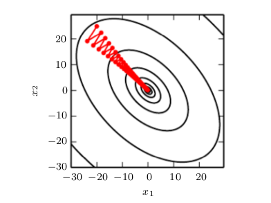
Gradient descent fails to exploit the curvature information contained in the Hessian matrix. Here we use gradient descent to minimize a quadratic function f( x ) whose Hessian matrix has condition number 5. This means that the direction of most curvature has five times more curvature than the direction of least curvature. In this case, the most curvature is in the direction [1,1] and the least curvature is in the direction [1, −1] . The red lines indicate the path followed by gradient descent. This very elongated quadratic function resembles a long canyon. Gradient descent wastes time repeatedly descending canyon walls, because they are the steepest feature. Because the step size is somewhat too large, it has a tendency to overshoot the bottom of the function and thus needs to descend the opposite canyon wall on the next iteration. The large positive eigenvalue of the Hessian corresponding to the eigenvector pointed in this direction indicates that this directional derivative is rapidly increasing, so an optimization algorithm based on the Hessian could predict that the steepest direction is not actually a promising search direction in this context.

This issue can be resolved by using information from the Hessian matrix to guide the search. The simplest method for doing so is known as Newton’s method. Newton’s method is based on using a second-order Taylor series expansion to approximate f ( x ) near some point x (0) :

$$ f(x) \approx f(x^0) + (x-x^0)^T \triangledown_x f(x^0) + \frac {1} {2} (x-x^0)^T H_f(x^0)(x-x^0)

$$

If we then solve for the critical point of this function, we obtain:

$$ x^* = x^0 - \triangledown_x f(x^0) H_f(x^0)^{-1}

$$

When f is a positive definite quadratic function, Newton’s method consists of applying Eq. 4.12 once to jump to the minimum of the function directly. When f is not truly quadratic but can be locally approximated as a positive definite quadratic, Newton’s method consists of applying Eq. 4.12 multiple times. Iteratively updating the approximation and jumping to the minimum of the approximation can reach the critical point much faster than gradient descent would. This is a useful property near a local minimum, but it can be a harmful property near a saddle point. As discussed in Sec. 8.2.3 , Newton’s method is only appropriate when the nearby critical point is a minimum (all the eigenvalues of the Hessian are positive), whereas gradient descent is not attracted to saddle points unless the gradient points toward them.

Optimization algorithms such as gradient descent that use only the gradient are called first-order optimization algorithms. Optimization algorithms such as Newton’s method that also use the Hessian matrix are called second-order optimization algorithms (Nocedal and Wright , 2006 ).