Deep Feedforward Networks
Deep feedforward networks , also often called feedforward neural networks , or multi-layer perceptrons ( MLPs ), are the quintessential deep learning models. The goal of a feedforward network is to approximate some function $$f^$$ . For example, for a classifier, $$y = f^(x)$$ maps an input x to a category y. A feedforward network defines a mapping y = f (x; θ) and learns the value of the parameters θ that result in the best function approximation.
Feedforward neural networks are called networks because they are typically represented by composing together many different functions. The model is associated with a directed acyclic graph describing how the functions are composed together. For example, we might have three functions $$f^{(1)}, f^{(2)}, f^{(3)}$$ connected in a chain, to form $$f(x) = f^{(1)}(f^{(2)}(f^{(3)}(x)))$$. These chain structures are the most commonly used structures of neural networks. In this case, f (1) is called the first layer of the network, f (2) is called the second layer, and so on. The overall length of the chain gives the depth of the model. It is from this terminology that the name “deep learning” arises. The final layer of a feedforward network is called the output layer. During neural network training, we drive f(x) to match $$f^(x)$$. The training data provides us with noisy, approximate examples of $$f^(x)$$ evaluated at different training points. Each example x is accompanied by a label $$y \approx f^(x)$$. The training examples specify directly what the output layer must do at each point x; it must produce a value that is close to y. The behavior of the other layers is not directly specified by the training data. The learning algorithm must decide how to use those layers to produce the desired output, but the training data does not say what each individual layer should do. Instead, the learning algorithm must decide how to use these layers to best implement an approximation of f∗ . Because the training data does not show the desired output for each of these layers, these layers are called hidden layers. Finally, these networks are called neural because they are loosely inspired by neuroscience. Each hidden layer of the network is typically vector-valued. The dimensionality of these hidden layers determines the width of the model. Each element of the vector may be interpreted as playing a role analogous to a neuron. Rather than thinking of the layer as representing a single vector-to-vector function, we can also think of the layer as consisting of many units that act in parallel, each representing a vector-to-scalar function. Each unit resembles a neuron in the sense that it receives input from many other units and computes its own activation value. The idea of using many layers of vector-valued representation is drawn from neuroscience. The choice of the functions $$f^{(i)}(x)$$used to compute these representations is also loosely guided by neuroscientific observations about the functions that biological neurons compute. However, modern neural network research is guided by many mathematical and engineering disciplines, and the goal of neural networks is not to perfectly model the brain. It is best to think of feedforward networks as function approximation machines that are designed to achieve *statistical generalization, occasionally drawing some insights from what we know about the brain, rather than as models of brain function.
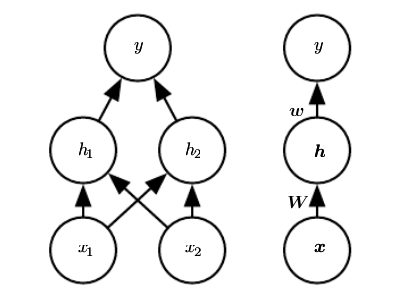
To extend linear models to represent nonlinear functions of x, we can apply the linear model not to x itself but to a transformed input $$\phi(x)$$, where $$\phi$$ is a nonlinear transformation. We can think of $$\phi$$ as providing a set of features describing x, or as providing a new representation for x . The strategy of deep learning is to learn $$\phi$$. In this approach, we have a model $$y = f(x;\theta, w) = \phi(x;\theta)^Tw$$. We now have parameters θ that we use to learn $$\phi$$ from a broad class of functions, and parameters w that map from $$\phi(x)$$ to the desired output. This is an example of a deep feedforward network, with $$\phi$$ defining a hidden layer. This approach gives up on the convexity of the training problem, but the benefits outweigh the harms. In this approach, we parametrize the representation as $$\phi(x; θ)$$and use the optimization algorithm to find the θ that corresponds to a good representation. If we wish, this approach can be highly generic—we do so by using a very broad family $$\phi(x; θ)$$. This approach can also let human practitioners encode their knowledge to help generalization by designing families $$\phi(x; θ)$$ that they expect will perform well. The advantage is that the human designer only needs to find the right general function family rather than finding precisely the right function.
They form the basis of many important commercial applications. For example, the convolutional networks used for object recognition from photos are a specialized kind of feedforward network.
When feedforward neural networks are extended to include feedback connections, they are called recurrent neural networks, which power many natural language applications.
Terms
- statistical generalization
- feature space
a model that learns a different feature space
An affine transformation is any transformation that preserves collinearity (i.e., all points lying on a line initially still lie on a line after transformation) and ratios of distances (e.g., the midpoint of a line segment remains the midpoint after transformation).
affine transformation controlled by learned parameters, followed by a fixed, nonlinear function called an activation function
Learning XOR Function
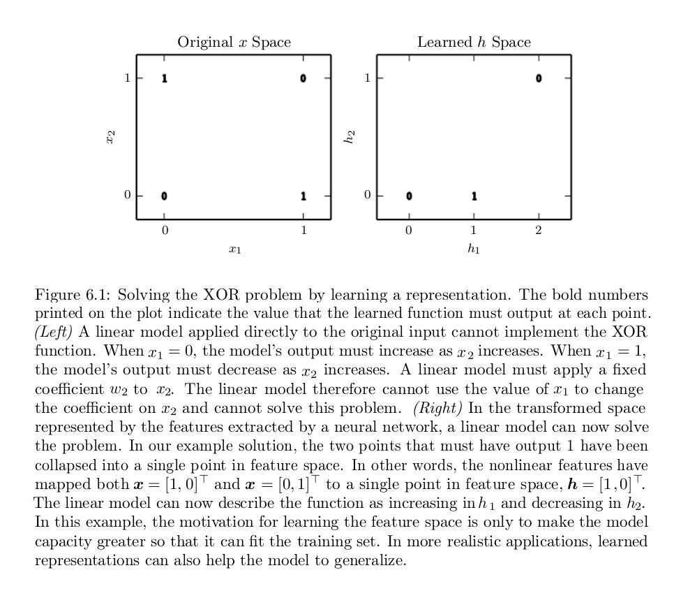
The XOR function provides the target function $$y = f^(x)$$ that we want to learn. Our model provides a function y = f(x;θ ) and our learning algorithm will adapt the parameters θ to make f as similar as possible to $$f^$$. In this simple example, we will not be concerned with statistical generalization. We want our network to perform correctly on the four points $$X = {(0,0)^T, (0,1)^T, (1,0)^T, (1,1)^T }$$. We will train the network on all four of these points. The only challenge is to fit the training set.
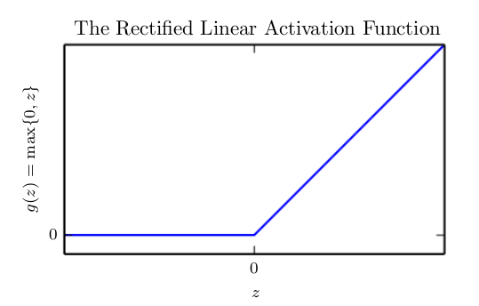
Clearly, we must use a nonlinear function to describe the features. Most neural networks do so using an affine transformation controlled by learned parameters, followed by a fixed, nonlinear function called an activation function. We use that strategy here, by defining $$h = g(W^Tx+c)$$, where W provides the weights of a linear transformation and c the biases. The activation function g is typically chosen to be a function that is applied element-wise, with $$hi = g(x^TW:i+c_i)$$. In modern neural networks, the default recommendation is to use the rectified linear unit or ReLU, defined by the activation function $$g(z) = max(0,z)$$.

The rectified linear activation function. This activation function is the default activation function recommended for use with most feedforward neural networks. Applying this function to the output of a linear transformation yields a nonlinear transformation. However, the function remains very close to linear, in the sense that is a piecewise linear function with two linear pieces. Because rectified linear units are nearly linear, they preserve many of the properties that make linear models easy to optimize with gradient-based methods. They also preserve many of the properties that make linear models generalize well. A common principle throughout computer science is that we can build complicated systems from minimal components. Much as a Turing machine’s memory needs only to be able to store 0 or 1 states, we can build a universal function approximator from rectified linear functions.

We can now specify our complete network for XOR function as $$f(x; W, c, w, b) = w^Tg((W^Tx+c))+b$$